I exercise the Chakravaty growth model in Excel. (Computational Economics, David A. Kendrick, P. Ruben Mer ,Hans M. Amman.) In that model we can obtain steady-state value for capital by solve a Hamiltonian problem or Azariadis approach.
k(ss)= (rho/(alpha*theta))^(1/alpha -1)in which
rho=(1-*betha)/betha)
is discount factor and
y = theta*(k^alpha)
After this, I try to run a growth model in gams. For this, I read (or run): "An Elementary Ramsey Growth Model" By : Kalvelagan "Neo-clasical/Ramsey model of Optimal Economic Growth" "A simple one sector Ramsey-type model" "Calibration of models with multi-years period",by you and two library gams model(Chakravaty and Ramsey) after this I contact with you and read papers that you suggest.
In all of this steps I want to find the steady-state value for capital as terminal condition. After your email, I find that terminal condition maybe diffrent from my imagination (and find this on Kalevelagan paper and in your massage) .
I(tlast)=(g+delta) * K(tlast)
and the discount factor for first steady-state priod is:
(1+rho)^(-t) t not last(t)
(rho^-1)*((1+rho)^(1-t)) t last(t)
In model that you reform for me, you have
beta(tnotlast(t)) = ((1+g)^etha/(1+rho))^t
If I don't make a mistake,
beta(tlast(t)) = (rho^-1)*((1+rho)/(1+g)^etha)^(1-t)
It is true?
I attached the GAMS file that adds terminal condition. Thanks a lot. Excuse me for my bad english for taking your time.
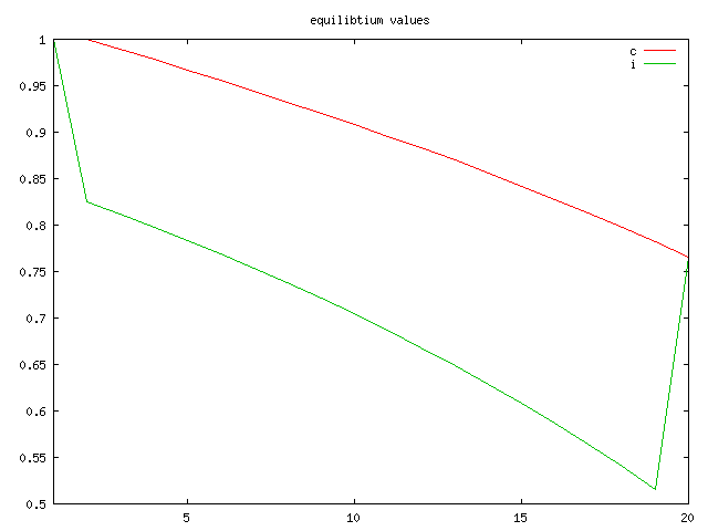
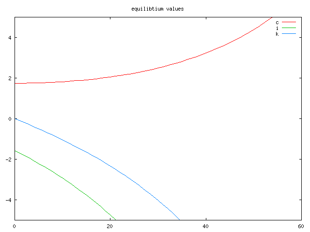
Your model does not place an appropriate welfare weight on the final period consumption (see the highlighted assignment below). You have also specified too short a model horizon which produces a a very poor approximation to the calibrated steady-state growth path:
The model works fairly well for the first 20 years if you set a 200 year horizon (simply define set t as "/t1*t200/"):
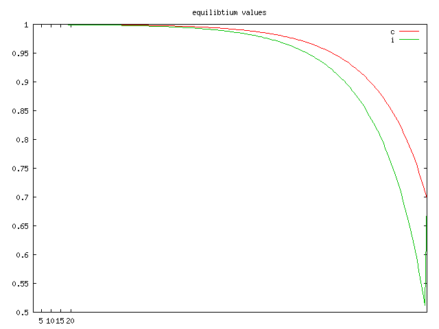
As you can see, it is a simple matter to identify a problem with the terminal approximation -- simply increase the time horizon and see if the model results are robust.
The use of finite-dimensional numerical methods to solve infinite-horizon growth models demands that you pay attention to the nature of the economic shock you are applying, as the magnitude of the shock determines the number of years over which you will need to run the model. It is for this reason that termination methods are quite important, as if you use a better terminal approximation, you do not need to run the model as many years into the future.
I've written out some notes on the underlying ideas, and here are the accompanying Figures 1-3.
$TITLE growth model with invalid terminal approximation
sets t time periods /t1*t20/;
scalars g labour growth rate /0.023/
delta depreciation /0.04 /
I0 initial investment /0.30 /
c0 initial consumption /0.27 /
b capital value share /0.65 /
etha inverse intertemporal elasticity / 2 /
rho marginal product of capital
k0 initial capital
l0 initial labour
a cobb douglas scale parameter;
sets
tfirst(t) first period
tlast(t) last period
tnotlast(t) all but last ;
tfirst(t)$(ord(t)=1)=yes;
tlast(t)$(ord(t)=card(t))=yes;
tnotlast(t)=not tlast(t);
parameters
l(t) labour
beta(t) weight factor of capital
tval(t) numerical value of t ;
tval(t)=ord(t)-1;
k0 = i0/(g+delta);
rho = b*(c0+i0)/k0-delta;
display rho;
l0 = (1-b)*(c0+i0);
beta(tnotlast(t))= power((1+rho)/(1+g)**etha,-tval(t));
beta(tlast(t))=(1/rho)*power((1+rho)/(1+g)**etha,1-tval(t));
a = (c0+i0)/(k0**b*l0**(1-b));
l(t) = power(1+g,tval(t))*l0;
variables
c(t) consumption
k(t) capital stock
y(t) production
I(t) investment
w intertemporal utility;
equations
production cobb douglas production function
allocation output market
accmulation capital stock evoluation
utility persent value of intertemporal walfare
final minimal invetment in lst period;
utility.. w =e= sum(t,beta(t)*(c(t)**(1-etha)))/(1-etha);
production(t).. y(t) =e= a*(k(t)**b)*(l(t)**(1-b));
allocation(t).. y(t) =g= c(t)+I(t);
accmulation(t+1).. k(t+1) =e= (1-delta)*k(t)+I(t);
final(tlast).. i(tlast) =g= (g+delta)*k(tlast);
c.l(t) = 1;
c.lo(t) = 0.01*c0;
k.lo(t) = 0.001;
c.fx(tfirst)= c0;
k.fx(tfirst) = k0;
I.lo(t) = 0;
model grm /all/;
option nlp=minos;
solve grm maximizing w using nlp;
parameter values(t,*) equilibtium values;
values(t,"c")= c.l(t)/(c0*power(1+g,tval(t)));
values(t,"i")= i.l(t)/(i0*power(1+g,tval(t)));
values(t,"c")= k.l(t)/(k0*power(1+g,tval(t)));
display values;
$TITLE Finite-Horizon Ramsey Growth Model with No Terminal Constraints
$if not set k0 $set k0 1
$if not set h $set h 100
sets t Time period (annual time steps) /0*%h%/,
tplot(t) Time periods for plotting /0*60/,
tl(tplot) Time periods for labelling /0 0, 20 20, 40 40, 60 60/;
scalars
g Labour growth rate in efficiency units /0.023/
delta Capital depreciation rate /0.04/
i0 Base year investment /0.30 /
c0 Base year consumption /0.27 /
b Capital value share /0.65 /
eta Inverse intertemporal elasticity / 2 /
rho Calibrated marginal product of capital,
k0 Initial capital
l0 Initial labour
a Cobb Douglas scale parameter;
sets tfirst(t) First period;
tfirst(t) = yes$(ord(t)=1);
parameters
qref(t) Steady-state output index
pref(t) Steady-state present value price index
l(t) Labour supply,
beta(t) Utility discount factor;
* Calibrate base year investment:
k0 = i0/(g+delta);
* Calibrate the base year marginal product of capital:
rho = b*(c0+i0)/k0-delta;
display rho;
pref(t) = power(1/(1+rho), ord(t)-1);
qref(t) = power(1+g,ord(t)-1);
abort$(g > rho) "Growth rate exceeds discount rate.",g,rho;
* Labor supply in the base year:
l0 = (1-b)*(c0+i0);
* Labor supply over the model horizon:
l(t) = l0 * qref(t);
* Utility discount parameter:
beta(t)= power((1+g)/(1+rho), ord(t)-1);
* Calibration of production scale parameter:
a = (c0+i0)/(k0**b * l0**(1-b));
variables
C(t) consumption
K(t) capital stock
Y(t) production
I(t) investment
W intertemporal utility;
equations
production cobb douglas production function
allocation output market
accmulation capital stock evoluation
utility persent value of intertemporal walfare;
utility.. W =e= sum(t, beta(t) * (C(t)/(c0*qref(t)))**(1-eta)) /(1-eta);
production(t).. Y(t) =e= a * K(t)**b * l(t)**(1-b);
allocation(t).. Y(t) =g= C(t) + I(t);
accmulation(t+1).. K(t+1) =e= (1-delta)*K(t) + I(t);
C.l(t) = c0 * qref(t);
K.l(t) = k0 * qref(t);
C.lo(t) = 0.01 * C.l(t);
I.lo(t) = 0;
K.lo(t) = 0;
K.fx(tfirst) = k0 * %k0%;
model grm /all/;
solve grm maximizing w using nlp;
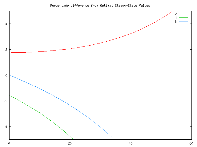
parameter values(t,*) Percentage difference from Optimal Steady-State Values;
values(t,"c")= 100 * (c.l(t)/(c0*qref(t)) - 1) + eps;
values(t,"i")= 100 * (i.l(t)/(i0*qref(t)) - 1) + eps;
values(t,"k")= 100 * (k.l(t)/(k0*qref(t)) - 1) + eps;
display values;
$setglobal domain tplot
$setglobal labels tl
$setglobal gp_opt0 'set yrange [-5:5]'
$if not set noplot $libinclude plot values
$TITLE Finite-Horizon Ramsey Growth Model with a Counter-Productive Terminal Constraint
$if not set k0 $set k0 1
$if not set h $set h 100
sets t Time period (annual time steps) /0*%h%/,
tplot(t) Time periods for plotting /0*60/,
tl(tplot) Time periods for labelling /0 0, 20 20, 40 40, 60 60/;
scalars
g Labour growth rate in efficiency units /0.023/
delta Capital depreciation rate /0.04/
i0 Base year investment /0.30 /
c0 Base year consumption /0.27 /
b Capital value share /0.65 /
eta Inverse intertemporal elasticity / 2 /
rho Calibrated marginal product of capital,
k0 Initial capital
l0 Initial labour
a Cobb Douglas scale parameter;
sets tfirst(t) First period,
tlast(t) Last period;
tfirst(t) = yes$(ord(t)=1);
tlast(t) = yes$(ord(t)=card(t));
parameters
qref(t) Steady-state output index
pref(t) Steady-state present value price index
l(t) Labour supply,
beta(t) Utility discount factor;
* Calibrate base year investment:
k0 = i0/(g+delta);
* Calibrate the base year marginal product of capital:
rho = b*(c0+i0)/k0-delta;
display rho;
pref(t) = power(1/(1+rho), ord(t)-1);
qref(t) = power(1+g,ord(t)-1);
abort$(g > rho) "Growth rate exceeds discount rate.",g,rho;
* Labor supply in the base year:
l0 = (1-b)*(c0+i0);
* Labor supply over the model horizon:
l(t) = l0 * qref(t);
* Utility discount parameter:
beta(t)= power((1+g)/(1+rho), ord(t)-1);
* Calibration of production scale parameter:
a = (c0+i0)/(k0**b * l0**(1-b));
variables
C(t) consumption
K(t) capital stock
Y(t) production
I(t) investment
W intertemporal utility;
equations
production Cobb Douglas production function,
allocation Output market,
accmulation Capital stock evoluation,
terminvest Terminal investment,
utility Intertemporal walfare;
utility.. W =e= sum(t, beta(t) * (C(t)/(c0*qref(t)))**(1-eta)) /(1-eta);
production(t).. Y(t) =e= a * K(t)**b * l(t)**(1-b);
allocation(t).. Y(t) =g= C(t) + I(t);
accmulation(t+1).. K(t+1) =e= (1-delta)*K(t) + I(t);
terminvest(tlast).. I(tlast) =g= (g+delta) * K(tlast);
C.l(t) = c0 * qref(t);
K.l(t) = k0 * qref(t);
C.lo(t) = 0.01 * C.l(t);
I.lo(t) = 0;
K.lo(t) = 0;
K.fx(tfirst) = k0 * %k0%;
model grm /all/;
solve grm maximizing w using nlp;
parameter values(t,*) equilibtium values;
values(t,"c")= 100 * (c.l(t)/(c0*qref(t)) - 1) + eps;
values(t,"i")= 100 * (i.l(t)/(i0*qref(t)) - 1) + eps;
values(t,"k")= 100 * (k.l(t)/(k0*qref(t)) - 1) + eps;
display values;
$setglobal domain tplot
$setglobal labels tl
$setglobal gp_opt0 'set yrange [-5:5]'
$if not set noplot $libinclude plot values
$TITLE Finite-Horizon Ramsey Growth Model with Manne-Barr Terminal Constraint
$if not set h $set h 100
$if not set k0 $set k0 1
sets t Time period (annual time steps) /0*%h%/,
tplot(*) Time periods for plotting /0*60/,
tl(tplot) Time periods for labelling /0 0, 20 20, 40 40, 60 60/;
scalars
g Labour growth rate in efficiency units /0.023/
delta Capital depreciation rate /0.04/
i0 Base year investment /0.30 /
c0 Base year consumption /0.27 /
b Capital value share /0.65 /
eta Inverse intertemporal elasticity / 2 /
rho Calibrated marginal product of capital,
k0 Initial capital
l0 Initial labour
a Cobb Douglas scale parameter;
sets tfirst(t) First period,
tlast(t) Last period;
tfirst(t) = yes$(ord(t)=1);
tlast(t) = yes$(ord(t)=card(t));
parameters
qref(t) Steady-state output index
pref(t) Steady-state present value price index
l(t) Labour supply,
beta(t) Utility discount factor;
* Calibrate base year investment:
k0 = i0/(g+delta);
* Calibrate the base year marginal product of capital:
rho = b*(c0+i0)/k0-delta;
display rho;
pref(t) = power(1/(1+rho), ord(t)-1);
qref(t) = power(1+g,ord(t)-1);
abort$(g > rho) "Growth rate exceeds discount rate.",g,rho;
* Labor supply in the base year:
l0 = (1-b)*(c0+i0);
* Labor supply over the model horizon:
l(t) = l0 * qref(t);
* Utility discount parameter:
beta(t)= power((1+g)/(1+rho), ord(t)-1);
* sum_{t=0}^inf a**t = 1/(1-a)
beta(tlast) = beta(tlast) * (1+rho)/(rho-g);
* Calibration of production scale parameter:
a = (c0+i0)/(k0**b * l0**(1-b));
variables
C(t) consumption
K(t) capital stock
Y(t) production
I(t) investment
W intertemporal utility;
equations
production Cobb Douglas production function,
allocation Output market,
accmulation Capital stock evoluation,
terminvest Terminal investment,
utility Intertemporal walfare;
utility.. W =e= sum(t, beta(t) * (C(t)/(c0*qref(t)))**(1-eta)) /(1-eta);
production(t).. Y(t) =e= a * K(t)**b * l(t)**(1-b);
allocation(t).. Y(t) =g= C(t) + I(t);
accmulation(t+1).. K(t+1) =e= (1-delta)*K(t) + I(t);
terminvest(tlast).. I(tlast) =g= (g+delta) * K(tlast);
C.l(t) = c0 * qref(t);
K.l(t) = k0 * qref(t);
C.lo(t) = 0.01 * C.l(t);
I.lo(t) = 0;
K.lo(t) = 0;
K.fx(tfirst) = k0 * %k0%;
model grm /all/;
solve grm maximizing w using nlp;
parameter values(t,*) equilibtium values;
values(t,"c")= 100 * (c.l(t)/(c0*qref(t)) - 1) + eps;
values(t,"i")= 100 * (i.l(t)/(i0*qref(t)) - 1) + eps;
values(t,"k")= 100 * (k.l(t)/(k0*qref(t)) - 1) + eps;
display values;
$setglobal domain tplot
$setglobal labels tl
*$setglobal gp_opt0 'set yrange [-5:5]'
$if not set noplot $libinclude plot values
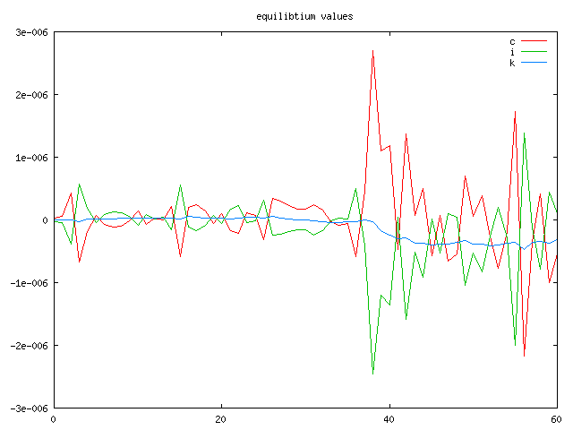
$TITLE Finite-Horizon Ramsey Growth Model in MCP Format
$if not set h $set h 100
$if not set k0 $set k0 1
* k0=%k0% h=%h%
sets t Time period (annual time steps) /0*%h%/,
tplot(*) Time periods for plotting /0*60/,
tl(tplot) Time periods for labelling /0 0, 20 20, 40 40, 60 60/;
scalars
g Labour growth rate in efficiency units /0.023/
delta Capital depreciation rate /0.04/
i0 Base year investment /0.30 /
c0 Base year consumption /0.27 /
b Capital value share /0.65 /
eta Inverse intertemporal elasticity / 2 /
rho Calibrated marginal product of capital,
k0 Initial capital
l0 Initial labour
a Cobb Douglas scale parameter;
sets tfirst(t) First period,
tlast(t) Last period;
tfirst(t) = yes$(ord(t)=1);
tlast(t) = yes$(ord(t)=card(t));
parameters
qref(t) Steady-state output index
pref(t) Steady-state present value price index
l(t) Labour supply,
beta(t) Utility discount factor;
* Calibrate base year investment:
k0 = i0/(g+delta);
* Calibrate the base year marginal product of capital:
rho = b*(c0+i0)/k0-delta;
display rho;
pref(t) = power(1/(1+rho), ord(t)-1);
qref(t) = power(1+g,ord(t)-1);
abort$(g > rho) "Growth rate exceeds discount rate.",g,rho;
* Labor supply in the base year:
l0 = (1-b)*(c0+i0);
* Labor supply over the model horizon:
l(t) = l0 * qref(t);
* Utility discount parameter:
beta(t)= power((1+g)/(1+rho), ord(t)-1);
* Calibration of production scale parameter:
a = (c0+i0)/(k0**b * l0**(1-b));
scalar svtarget Switch for state-variable targetting /0/;
variables
C(t) consumption
K(t) capital stock
Y(t) production
I(t) investment
W intertemporal utility;
equations
production Cobb Douglas production function,
allocation Output market,
accmulation Capital stock evoluation,
utility Intertemporal walfare;
utility.. W =e= sum(t, beta(t) * (C(t)/(c0*qref(t)))**(1-eta)) /(1-eta);
production(t).. a * K(t)**b * l(t)**(1-b) =E= Y(t);
allocation(t).. Y(t) =g= C(t) + I(t);
accmulation(t).. (1-delta)*K(t-1) + I(t-1) + (k0*%k0%)$tfirst(t) =e= K(t);
C.l(t) = c0 * qref(t);
K.l(t) = k0 * qref(t);
C.lo(t) = 0.01 * C.l(t);
I.lo(t) = 0;
K.lo(t) = 0.01 * K.L(t);
model grm /all/;
solve grm maximizing w using nlp;
VARIABLES PY(t) Shadow value of output,
P(t) Shadow value of market supply,
PK(t) Shadow value of capital,
PKT(t) Salvage value of capital;
PY.L(t) = -production.m(t);
P.L(t) = -allocation.m(t);
PK.L(t) = -accmulation.m(t);
EQUATIONS FOC_Y,FOC_C,FOC_I,FOC_K,KT;
FOC_Y(t).. PY(t) =E= P(t);
FOC_C(t).. P(t) =E= beta(t) * C(t)**(-eta) / (c0*qref(t))**(1-eta);
FOC_I(t).. P(t) =G= PK(t+1) + PKT(t)$tlast(t);
FOC_K(t).. PK(t) =E= b * PY(t) * a * K(t)**(b-1) * l(t)**(1-b) + (1-delta) * (PK(t+1)+PKT(t)$tlast(t));
KT(tlast).. sum(t$tlast(t), I(t) - (1+g) * I(t-1))$svtarget +
(I(tlast) - (g+delta) * K(tlast))$(not svtarget) =E= 0;
model grm_mcp / production.PY,allocation.P,accmulation.PK,
FOC_Y.Y, FOC_C.C, FOC_I.I, FOC_K.K, KT.PKT /;
* Solve first without state-variable targetting to improve robustness:
PKT.LO(tlast) = -inf;
PKT.UP(tlast) = +inf;
grm_mcp.iterlim = 10000;
solve grm_mcp using mcp;
* Then solve with the more precise terminal constraint:
svtarget = 1;
solve grm_mcp using mcp;
parameter values(t,*) equilibtium values;
values(t,"c")= 100 * (c.l(t)/(c0*qref(t)) - 1) + eps;
values(t,"i")= 100 * (i.l(t)/(i0*qref(t)) - 1) + eps;
values(t,"k")= 100 * (k.l(t)/(k0*qref(t)) - 1) + eps;
display values;
$setglobal domain tplot
$setglobal labels tl
$setglobal gp_opt0 'set yrange [-1e-5:1e-5]'
$if not set noplot $libinclude plot values